Macro-Actions Quick Overview
This post will serve as a mini survey of macro-actions and MacDec-POMDPs.
What is a Macro-Action
A macro-action is essentially a high-level action. It is based off the options framework and is essentially hierarchical reinforcement learning [4]. The options framework is temporally extracted actions like “skills/macros” in the single agent case. Macro-actions which can be also called options are an extension of that by framing it as a Dec-POMDP problem which makes it multi-agent. This is formally coined as a MacDec-POMDP. Options, however, are synchronous and agents need to be homogeneous. We are learning high-level policies over macro-actions which maps histories to macro-actions. A macro-action allows agents to have the ability to asynchronously learn to collaborate with another through a multi-agent reinforcement learning lens. The macro-action is defined as $m = \langle \beta_m, I_m, \pi_m \rangle$ (based off the options framework). $\beta_m$ is the stochastic termination condition where at each history conditioned on the observation, there is a chance for the macro-action to terminate. $I_m$ is the initiation set that needs to be met from the macro-observation-history for the macro-action to start. $\pi_m$ is the low-level policy ran to successfully execute the macro-action.
To recap, the reason why we use macro-actions is for a way to represent agent coordination in a more simple and realistic manner. In the real world, robots/agents are not all homogenous and they are never synchronized to finish their task at the exact same time. So, the main difference between options and macro-action is the fact that we are now solving a Dec-POMDP rather than a POMDP, allow for macro-actions that run for different timesteps, allow for asynchronous execution, reduces complexity of planning in long horizon tasks, and improve agent collaboration. Moreover, macro-actions that build on top of other macro-actions would allow for more complex hierarchical planning as well.
A MacDec-POMDP [1, 2] is defined as the tuple:
\[\langle I, S, A, M, \Omega, \zeta, T, R, O, Z, \mathbb{H}, \gamma \rangle\]The tuple $\langle I, S, A, \Omega, O, R \rangle$ in MacDec-POMDP are from the definition of Dec-POMDP.
$I$ represents a set of agents;
$S$ defines the environmental state space;
$A = \prod_{i \in I} A_i$ denotes the combined primitive-action space, from each agent’s individual primitive-action set $A_i$;
$M = \prod_{i \in I} M_i$ indicates the joint macro-action space, comprising each agent’s macro-action space $M_i$;
$\Omega = \prod_{i \in I} \Omega_i$ describes the joint primitive-observation space, combining each agent’s primitive-observation set $\Omega_i$;
$ Z = \prod_{i \in I} Z_i$ represents the joint macro-observation space, which combines each agent’s macro-observation space $\zeta_i$;
$T(s, \vec{a}, s’) = P(s’ \mid s, \vec{a})$ explains the environment transition dynamics;
$R(s, \vec{a})$ serves as the global reward function. Reward comes from the underlying ground truth environment state.
$\mathbb{H}$ is the horizon;
$\gamma$ is the discount variable.
When using macro-actions, each agent independently selects a macro-action based on the high level policy and collects a macro-observation. The objective of solving MacDec-POMDPs with a finite horizon is finding a joint high-level policy $\vec{\Psi} = \prod_{i \in I} \Psi_i$ that maximizes the value:
\[V^{\vec{\Psi}}(s_{(0)}) = \mathbb{E}\!\left[\sum_{t=0}^{\mathbb{H}-1} \gamma^t\, r\!\left(s_{(t)}, \vec{a}_{(t)}\right) \;\middle|\; s_{(0)}, \vec{\pi}, \vec{\Psi}\right]\]where $\gamma \in [0,1]$ is the discount, and $\mathbb{H}$ is the number of time steps until the problem terminates. It is important to note that there is no individual reward/credit assignment in a MacDec-POMDP or Dec-POMDP. It only uses a team reward which promotes collaboration as each agent’s actions will affect the team reward and we are maximizing the overall team reward. The problem when there are individual rewards is called a POSG (partially observable stochastic game) [9]. You could solve a POSG using a formulation with POMDP because a single agent POSG can be modeled as a POMDP. However, since games like chess are two-agents, it would need further techniques to make this work. Since POSG is not the main topic here, I will not talk more about it.
Notation and Function Definitions
These are the common functions and notations that you would probably see in a macro-action paper.
\[\begin{aligned} Q^{\theta_i}_{\phi_i}(h_i, m_i) \quad & \text{is the decentralized critic} \\ Q^{\vec{\Psi}}_{\phi}(\vec{h}, \vec{m}) \quad & \text{is the centralized critic} \\ \Psi_{\theta_i}(m_i \mid h_i) \quad & \text{is the macro-action-based policy and is the individual actor} \\ \Psi_{\theta}(\vec{m} \mid \vec{h}) \quad & \text{is the centralized actor or joint macro-action-based policy} \\ V^{\Psi_{\theta_i}}_{\mathbf{w}_i}(h_i) \quad & \text{is the local history value function or critic} \\ V^{\Psi_{\theta}}_{\mathbf{w}}(\vec{h}) \quad & \text{is the centralized history value function or critic} \\ V^{\vec{\Psi}_{\theta_i}}_{\mathbf{w}_i}(\vec{h}_i) \quad & \text{is the separate centralized critic used in MAPPO} \\ r_i^c \quad & \text{is the cumulative-discounted reward of the macro-action taking } \tau_{mi} \text{ time steps} \\ Q_{\phi_i}(h_i, m_i) \quad & \text{is the individual macro-action-value function} \\ Q_{\phi_i}(\vec{h}_i, \vec{m}_i) \quad & \text{is the joint macro-action value function} \\ x \quad & \text{represents the available centralized information} \\ \vec{A} \quad & \text{advantage calculated using centralized information using GAE} \\ \alpha \quad & \text{is the positive coefficient for clipping function} \\ \beta \quad & \text{is the negative coefficient for the clipping function} \\ \end{aligned}\]Discrete Macro-Actions
Currently, most research is on discrete macro-actions where we assume that the macro-action itself is a discrete high-level action such as “go-to-point-A” or “go-to-kitchen” [5,6,7,8]. The low level policy/controller will then run the primitive actions or trajectory planner that will achieve that goal. As many can realize, this is a form of hierarchical reinforcement learning. I will discuss about the continuous extension briefly in the later sections. For this section, I will focus mostly on current macro-action algorithms from my knowledge. I am fairly confident the following are 90%+ of all the current macro-action algorithms.
Early Work (2014-2017)
First, I will talk about the solution to a MacDec-POMDP which I briefly mentioned above. As mentioned previously, the solution maps option/macro-action histories to macro-actions. An option/macro-option history is formally defined as $h^M_{i} = (z^0_i, m^1_i,…, z^{t-1}_i, m^{t-1}_i)$ where $M$ is the macro-action and $i$ is the agent number. It is important to note here that we are counting the number of macro-actions as each macro-action can last different number of primitive time steps depending on the low-level/sub policy. The stochastic policy of each agent using macro-action is then defined as $\mu_i: H_i^M \times M_i \to [0, 1]$ which depends on the joint observation and joint policy $\mu$. Then, the goal would be to maximize the joint high-level policy as stated above in the first section.
An early solution of finding the optimal high-level policy or macro-action policy is using dynamic programming called Option-based Dynamic Programming (O-DP)[11]. This algorithm finds all possible combinations of macro-actions and chooses the best combination for the policy that returns the highest reward. This idea is then extended in Memory-bounded dynamic programming (MBDP) which does the same search but only retaining the best performing decision trees. Additionally, Option-based DIrect Cross Entropy (O-DICE) can also be used where it searches through the space of policy trees through sampling. It retains sampling distributions at each joint history and then evaluates them to get $V(h)$ so the best predefined number of policies are kept and worse ones removed.
These early solutions have policies as policy trees so the next extension of these algorithms is to represent them as finite-state controllers to be used in robotics [12]. The motivation for this extension is that finite-state controllers are easier to understand and much simpler than policy trees. The important part is that these finite-state controllers allow for infinite horizon planning as policy trees require the agent to remember the entire history which creates a memory problem when the horizon is infinite (needing infinite memory). Since this is modeled as a macro-action level, it only cares about the outcome of the macro-action and doesn’t care about the low-level execution. This greatly reduces the planning complexity because it doesn’t need to worry about all the possible trajectories and just chooses one. Then, it generates controllers for robots that maximizes the team reward. The planning algorithm that is able to do this is called MacDec-POMDP Heuristic Search (MDHS). The mathematical proofs for these simple algorithms will be omitted but can be seen in the papers referenced.
Recent Work (2017+)
More recently, we have better performing algorithms for this problem through the use of more modern reinforcement learning algorithms. These algorithms are from the single agent case but extended to the multi-agent case with macro-actions and provides a more principled way to solve the MacDec-POMDP problem compared to the brute force methods discussed previously. I will separate this to value-based methods and policy-gradient based methods. Moreover, these algorithms take advantage of the popular Centralized Training and Decentralized Execution (CTDE) paradigm. To explain CTDE briefly, we have centralized training and execution (CTE), decentralized training and execution (DTE), and CTDE. In CTE, the agents can all be representing as if it is one agent and is not any different from the single agent case aside from having joint observations and actions. This means that all the agents have information from the other agents as well. The DTE case differs as each agent acts independently and each have their own critic and actor and acts without any centralized information. CTDE combines both where in the training phase, information from all the agents can be used (in the centralized critic) in addition to any other underlying information if wanted but during execution, the agent only takes in its own local observations and executes its own actions (individual actors). Thus, we have a bellman equation for centralized macro-action based policy and decentralized macro-action based policy. A vector above the variable is used to represents joint.
The decentralized bellman equation is:
\[Q^{\Psi_i}(h_i, m_i) = \mathbb{E}_{h_i', \tau_i | h_i, m_i} \left[ r^c(h_i, m_i, \tau_i) + \gamma^{\tau_i} V^{\Psi_i}(h_i') \right] \quad\]The centralized bellman equation is:
\[Q^\Psi(\vec{h}, \vec{\mathbf{m}}) = \mathbb{E}_{\vec{h}', \tau | \vec{h}, \vec{\mathbf{m}}} \left[ \vec{r}^C(\vec{h}, \vec{\mathbf{m}}, \vec{\tau}) + \gamma^\tau V^\Psi(\vec{h}') \right] \quad\]An important addition in recent methods is the form of memory called Macro-Action Concurrent Experience Replay Trajectories (Mac-CERTS) and Macro-Action Joint Experience Replay (Mac-JERTs) [5]. These hold the individual and joint history information including the time information so that rewards for the macro-action are correctly collected in a sequential manner. More concretely, Mac-JERTS is where each agent accumulates the joint reward whenever the agent finishes its macro-action while Mac-CERTS collects the joint reward when any agent finishes its macro-action. This idea is difficult to write so it is easier to just visualize in figure 1 and 2. Mac-CERTS are used when we are training a decentralized macro-action value $Q_{\theta_i}$, while Mac-JERTS are used when training a centralized macro-action value $Q_{\phi}$ . Since macro-actions have varying timesteps until completion, we would discount by the number of macro-actions rather than at a certain timestep. So, through squeezing in Mac-JERTS and Mac-CERTS, we can record down when each macro-observation-history correctly to be used in more traditional reinforcement learning methods.
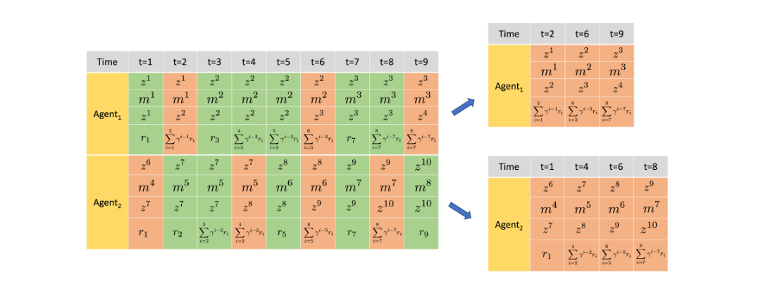
Figure 2. Example of Mac-CERTs. As you can see, each agent would accumulate the joint reward whenever they finish their own macro-action.
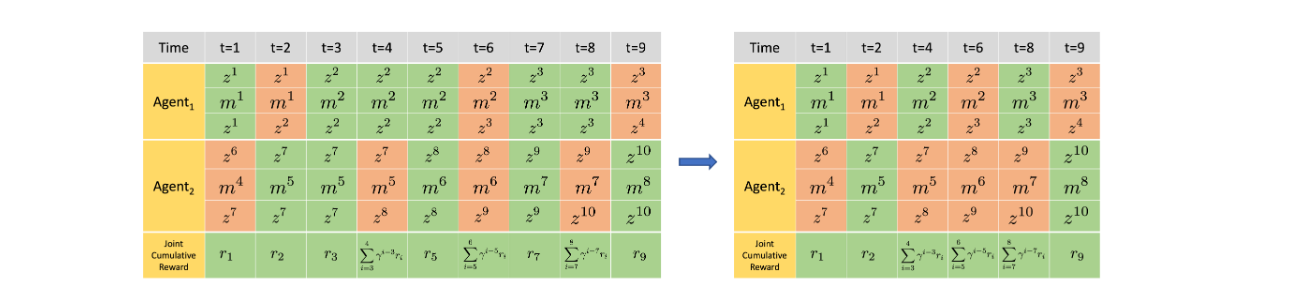
Figure 1. An example of Mac-JERTs. A joint sequential experience is first sampled from the memory buffer where the termination of each joint macro-action is represented in red and the non-termination in green. A squeezed sequential experience is generated for the centralized training is created by recording the joint history and joint reward whenever an agent terminates its macro-action.
Value-Based Methods
This idea is introduced along with the Deep Q-Networks (DQN)/ Deep Recurrent Q-Networks (DRQN) extension to macro-actions [13,14]. To explain briefly, DQN is a popular value-based method to update the policy $\pi$ by iteratively updating the action-value function, $Q(s,a)$. To extend DQN to the partially observable case, recurrent networks are introduced to remember some history of actions which is called DRQN. These algorithms adapted to the macro-action case are called Macro-Action Based Decentralized Multi-Agent Hysteretic Deep Recurrent Q-Networks (MacDec-MAHDRQN) and Macro-Action Based Decentralized Multi-Agent Hysteretic Double Deep Recurrent Q-Networks (MacDec-MAHDDRQN). In addition to the previous ones mentioned, MacDec-MAHDRQN and MacDec-MAHDDRQN also adds on the idea of hysteretic q-learning and double q-learning [15,16]. Hysteretic Q-learning is the same as traditional Q learning except we have an $\alpha$ and $\beta$ values where we use $\alpha$ which is the normal learning rate when our TD error is positive and $\beta$ when the TD error is negative. The basic idea is that negative TD error can be caused by another agent in the environment doing exploration and not domain stochasticity to avoid local optima in certain domains. So we want to use this to make each agent robust against negatively updating due to teammate mistakes/exploration. Afterall, other agents performing their policies in the environment causes the problem to be non-stationary in the local agent’s perspective learning in a decentralized manner with partially observability. The loss function for MacDec-MAHDDRQN is:
\[\mathcal{L}(\theta_i) = \mathbb{E}_{\langle \mathbf{z}, \mathbf{m}, \mathbf{z}', \mathbf{r}^c \rangle_i \sim \mathcal{D}} \left[ \left( y_i - Q_{\theta_i}(h, m) \right)^2 \right], \text{ where } y_i = r^c + \gamma^{\tau} Q_{\theta_i^-} \left( h', \arg \max_{\mathbf{m}'} Q_{\theta_i}(h', m') \right) \quad\]What is currently discussed is all the decentralized case. Luckily, the centralized case is very similar to the decentralized case and I will briefly explain centralized control. Essentially, in the centralized case, we have joint histories, rewards, macro-actions, etc. The loss function now in an example for centralized DDRQN is thus:
\[\mathcal{L}(\phi) = \mathbb{E}_{\langle \mathbf{z}, \mathbf{m}, \mathbf{z}', \mathbf{r}^c \rangle \sim \mathcal{D}} \left[ \left( y - Q_{\phi}(\vec{h}, \vec{m}) \right)^2 \right] \quad (19), \\ \text{ where } y_{(t)} = \bar{r}^C + \gamma Q_{\phi^-} \left( \vec{h}', \arg \max_{\vec{\mathbf{m}}'} Q_{\phi} \left( \vec{h}', \vec{\mathbf{m}}' \mid \vec{\mathbf{m}}^{\text{undone}} \right) \right) \quad\]Note that in the centralized case, since agents could still be continuing its macro-action while other agents terminate their macro-action, we need to have that conditional target prediction so our value estimates are more correct. Now we will move onto the CTDE case with Parallel Macro-Action-Based Decentralized Multi-Agent Double Deep Recurrent Q-Net (Parallel MacDec-MADDRQN).
Parallel Macro-Action-Based Decentralized Multi-Agent Double Deep Recurrent Q-Net (Parallel MacDec-MADDRQN) then improves on MacDec-MAHDRQN and MacDec-MAHDDRQN by addressing the problem of poor performance in larger domains. They still maintain decentralized execution as communication may be limited or none at times. As the method was experimented on robots, the macro-actions represented temporally extended robot controllers. Parallel MacDec-MADDRQN is derived from double DQN, but in this case, they train the centralized joint macro-action value $Q_{\phi}$ and each agent’s decentralized macro-action value function $Q_{\theta_i}$ in parallel. $Q_{\theta_i}$ is updated using information from $Q_{\phi}$ during training phase as centralized information is availiable and could be used for improved cooperation. The loss function for Parallel MacDec-MADDRQN is:
\[\mathcal{L}(\theta_i) = \mathbb{E}_{\mathbf{z}, \mathbf{m}, \mathbf{z}', \mathbf{r}^c, \vec{\mathbf{r}}^c \sim \mathcal{D}} \left[ \left( y_i - Q_{\theta_i}(h_i, m_i) \right)^2 \right] \quad, \\ \text{ where } y_i = r_i^c + \gamma Q_{\theta_i^-} \left[ h_i', \left[ \arg \max_{\mathbf{m}'} Q_{\phi}(\mathbf{h}', \mathbf{m}') \right]_i \right] \quad\]The difference between this loss function and the loss function from MacDec-MAHDDRQN (which is DTE) in this new algorithm is $\left[ \arg \max_{\mathbf{m}’} Q_{\phi}(\mathbf{h}’, \mathbf{m}’) \right]$. This means selecting the joint macro-action with the highest value and from that joint macro-action value, selecting the individual macro-action for agent $i$.
Policy-Gradient Methods
Next, we have policy-gradient based methods which are also based off the CTDE paradigm. These methods include Macro-Action Based Independent Actor Critic (Mac-IAC), Macro-Action Based Centralized Actor Critic (Mac-CAC), Macro-Action Based Independent Actor Independent Centralized Critic (Mac-IAICC), Macro-Action Based Multi-Agent Proximal Policy Optimization (Mac-MAPPO), and Macro-Action Based Independent Proximal Policy Optimiation(Mac-IPPO) [7,8]. Unlike value-based methods that update a Q-value, policy gradient methods update the network weights directly which means that it learns a stochastic policy. This could handle cases where deterministic policies might fail like in real world scenarios or situations where more exploration is needed. I will start with Macro-Action Based Independent Actor critic (Mac-IAC) where each agent independently trains its own actor and critic using its own local information. This means that other agents will be treated as part of the world which makes it look non-stationary in the local agent’s perspective which could result in low quality policies. The policy gradient update rule for the actor is then:
\[\nabla_{\theta_i} J(\theta_i) = \mathbb{E}_{\pi_{\theta}} \left[ \nabla_{\theta_i} \log \pi_{\theta_i}(a_i|h_i) \left( r + \gamma V_w^{\pi_{\theta_i}}(h_i') - V_w^{\pi_{\theta_i}}(h_i) \right) \right] \quad\]where $r$ is the team reward. Next, we have Macro-Action Based Centralized Actor Critic (Mac-CAC) where we train a single joint actor and joint critic with joint information and a cumulative joint reward $\vec{r}^c$:
\[\nabla_{\theta} J(\theta) = \mathbb{E}_{\Psi_{\theta}} \left[ \nabla_{\theta} \log \Psi_{\theta}(\vec{m} | \vec{h}) \left( \vec{r}^c + \gamma^{\vec{\tau}_{\vec{m}}} V_w^{\Psi_{\theta}}(\vec{h}') - V_w^{\Psi_{\theta}}(\vec{h}) \right) \right] \quad\]We will skip Macro-Action Based Independent Actor with Centralized Critic (Mac-IACC) as it is not correct and move onto Macro-Action Based Independent Actor Independent Centralized Critic (Mac-IAICC). Mac-IAICC is the correct formulation as it accumulates reward purely based on the execution of the agent $i$’s macro-action $m_i$ and not based on any random agent’s macro-action termination. This policy gradient is then:
\[\nabla_{\theta_i} J(\theta_i) = \mathbb{E}_{\Psi_{\vec{\theta}}} \left[ \nabla_{\theta_i} \log \Psi_{\theta_i}(m_i | h_i) \left( r_i^c + \gamma^{\tau_{m_i}} V_{w_i}^{\vec{\Psi}_{\vec{\theta}}}(x') - V_{w_i}^{\vec{\Psi}_{\vec{\theta}}}(x) \right) \right] \quad\]You might have noticed I didn’t mention the critic update rule. This is usually done using a mean squared error (MSE) loss. Finally, the most recent addition is the extension to MAPPO/IPPO[8]. The method Agent Centric Actor Critic (ACAC) is introduced for this purpose. It is essentially the extension of MAPPO to macro-actions. The contribution of this new method is by introducing an “agent-centric centralized critic”. This takes the place of using Mac-JERTS and Mac-CERTS by proposing an encoder that integrades the macro-observation with the timestep information using a self-attention module. The timestep information is embedded using a sinusoidal positional encoding and then combined with the macro-observation. The purpose of doing this is to represent the history more accurately. Mac-IPPO’s policy gradient can be repsented as:
\[\mathcal{L}(\theta_i) = \mathbb{E}_{m^{i}_t, h^{i}_t} \left[ \min \left( \frac{\Psi_{\theta_i}(m_i \mid h_i)}{\Psi_{\theta_{i,\text{old}}}(m_i \mid h_i)} A_t^{m_i}, \text{clip} \left( \frac{\Psi_{\theta_i}(m_i \mid h_i)}{\Psi_{\theta_{i,\text{old}}}(m_i \mid h_i)}, 1 - C, 1 + C \right) A_t^{m_i} \right) \right] \quad\] \[A_i = \sum_{t=t_{m_i}}^{t_{m_i} + T_{m_i} - 1} \gamma^{t - t_{m_i}} \delta_{t}^i \quad\] \[\delta = r_i^c + \gamma^{\tau_{m_i}} V_{w_i}^{\theta_i}(h_i') - V_{w_i}^{\theta_i}(h_i) \quad\]In this case, IPPO is fully decentralized (DTE). Following the idea of Mac-IAICC the MAPPO implementation where each agent has its own centralized critic is:
\[\mathcal{L}(\theta_i) = \mathbb{E}_{m^{i}_t, h^{i}_t} \left[ \min \left( \frac{\Psi_{\theta_i}(m_i \mid h_i)}{\Psi_{\theta_{i,\text{old}}}(m_i \mid h_i)} A_t^{m_i}, \text{clip} \left( \frac{\Psi_{\theta_i}(m_i \mid h_i)}{\Psi_{\theta_{i,\text{old}}}(m_i \mid h_i)}, 1 - C, 1 + C \right) A_t^{m_i} \right) \right] \quad\] \[A^{m_i}_i = \sum_{t=t_{m_i}}^{t_{m_i} + T_{m_i} - 1} \gamma^{t - t_{m_i}} \delta_{t}^i \quad\] \[\delta_{t}^i = r_i^c + \gamma^{\vec{\tau}_{\vec{m_i}}} V_{w_i}^{\vec{\psi}}(x') - V_{w_i}^{\vec{\psi}}(x) \quad\]As you can see, it is very similar to the IPPO actor update but we have the centralized critic with centralized history information rather than local history information in the advantage estimate. This makes it CTDE. This concludes the discrete macro-action section and start the new section that has not been formally introduced yet which is the concept of continuous macro-actions.
Continuous Macro Actions
Writing research paper on extending Macro-Actions to the continuous case. The main idea is that currently there is no formal definition for a continuous macro-action. The purpose of the continuous macro-action is similar to the reason for a continuous action; scalability. Let’s take an example of a mars rover exploring scientific points of interests. Instead of the discrete macro-action “go-to-point-A” it would be “go-to-location-(coordinates)”. This means that the macro-action is now a parameter (coordinates) that can be learned. The reason why we need continuous macro-action is for more realistic and refined control.
Let’s have an example with two rovers in a multi-agent scenario. We can assume they are homogenous agents with their macro-action/action space being the same. In this case, if both agents take the action to “go-to-point-A” and point A is this predefined position, it would collide with each other as they are trying to go to the same point and collect the same data. In the continuous case, they would be able to figure out they need to be side by side with one another or on opposite sides. In this case, they could both be at point A without collision of duplicate observations from the rover/agent’s perspective. More to be explained in later section.
Parameterized/Continuous Macro-Action
Reason/Motivation: It is mainly for scalability. If we use discrete macro-actions, and it is not parameterized, then for any large grid world, we would have a problem because it would be length × width amount of macro-actions to get to every point on the grid (same way of why we use continuous actions). With continuous macro-actions, we could solve that because we can learn the macro action that gets to where we want without having to store all the discrete macro-actions. This could translate to real-world control problems with robotics. There are many examples out there already on robots learning high-level actions in a hierarchical manner so they are able to collaborate with one another. What we are doing here is formalizing that in a MARL manner as a multi-agent way to do multi-robot collaboration in the real world.
Continuous Macro-Actions can have the underlying policy running discrete or continuous primitive actions. For the purpose of being succinct, we will just define the high-level policy in the continuous space but the lower-level policy will still be discrete. It is also possible to define both the high and low level policies to be continuous. In essence, high level is continuous but the lower level can be discrete or continuous.
Also real world robotics do not use discrete actions as robots can’t teleport to a place. It would need to move in continuous time to get to a certain area. We can form it in a way that looks discrete but the underlying actions are still continuous.
We can learn the termination condition by adding it to the MAPPO. Since the termination condition is learned, we can have macro-actions that can be more finely controlled. Other than the policy being continuous instead of discrete, the equations would remain the same.
Continuous Macro-Actions:
We assume that every continuous macro-action:
\[m\in\mathcal{M}\subset\mathbb{R}^d\]can be deterministically decomposed into a sequence of primitive actions in each agent’s primitive action set $\mathcal{A}_i \subset \mathbb{R}^k$. Concretely, there exists $(a_0, a_1, \dots, a_{\tau-1})$, where each
\[a_t \in A = \prod_{i \in I} A_i\]In this case, $\tau$ is the length of the macro-action. There is a deterministic map
\[\phi : A^\tau \longrightarrow \mathcal{M}, \qquad m = \phi(a_0, a_1, \dots, a_{\tau-1})\]During execution of $m$, at each underlying step $t=0,\dots,\tau-1$, the agent executes a discrete primitive action based on the local primitive observation history $H^A_i$. The macro-observation $z$ seen at macro-termination can itself be viewed as a function of the primitive observations: $\psi: \Omega^\tau \to \mathcal{Z}$.
Continuous macro-action as a Mac-DecPOMDP:
The idea is that it will randomly choose an ending point at some time step $t \mid h$. Learning policy over m as well as policy over b. I could say that previously it is predefined but now we assume it is not. I could write as two seperate functions or as one thing. I am not sure yet. When do I learn the termination function and when do I learn the other one? What would be the value if I stopped vs continued. These topics need to be explored more in the future.
When the option terminates (at primitive step $\tau_i$), there will be a new macro-observation $z^i$ via
\[Z_i\bigl(z^i\mid m^i,\,s_{\tau_i}\bigr) = P\bigl(z^i\mid h^i_{\tau_i},m^i\bigr)\]and its high-level macro-action observation history $h^i\in H^M_i$.
Under these definitions, we will have the high-level policy
\[\Psi_i\,(m^i\mid h^i),\quad m^i\in M_i\]becoming the density over options.
Problems?
- When objectives suddenly change like the box suddenly no longer exist in the preset position so it needs to cancel the macro-action and choose to go elsewhere. For example, we have box A and box B in certain positions but now box A and box B positions change.
- When other agents get to the objectives first like if turtlebot A outputs go to box A but turtlebot B also samples to go to box A but it gets there first. Then, turtlebot A would need to cancel the macro-action and sample another one. (This needs more thought. Some set of macro actions to do stuff but not the best.)
- Collaboration: turtlebot A goes to small box, but then it sees turtlebot B going into same area. Then both of them can cancel macro-action and sample at the same time a collaborative macro-action like go to big box since the big box can only be pushed with two turtlebots.
Learning Termination Condition
- $\beta_{m_i}(h^A_t) = Q(h,m) - V(h)$
- $Q(h,m’) - Q(h,m)$
Continuous Macro-Action Policy Gradient Theorem
Using Yuchen’s Macro-Action Policy Gradient Theorem as a base:
\[V^{\Psi}(h) = \int_{\mathcal{M}} \Psi(m\mid h)\, Q^{\Psi}(h, m)\, dm\](How good is $h$ over policy)
\[Q^{\Psi}(h, m) = r^c(h, m) + \int_{h'} P(h'\mid h, m)\, V^{\Psi}(h')\, dh'\](How good is taking macro-action over history)
where,
\[r^c(h, m) = \mathbb{E}_{\tau \sim \beta_m, s\mid_{t_m}}\biggl[\sum_{t=t_m}^{t_m+\tau-1} \gamma^t r_t\biggr]\] \[\begin{aligned} P(h'\mid h, m) &= P(z'\mid h, m) = \sum_{\tau=1}^{\infty} \gamma^{\tau} P\bigl(z', \tau \mid h, m\bigr) \\ &= \sum_{\tau=1}^{\infty} \gamma^{\tau} P\bigl(\tau\mid h, m\bigr) P\bigl(z'\mid h, m, \tau\bigr) \\ &= \mathbb{E}_{\tau \sim \beta_m}\,\Bigl[\gamma^{\tau}\, \mathbb{E}_{s\mid h}\bigl[\mathbb{E}_{s'\mid s,m,\tau}[\,P(z'\mid m,s')\,]\bigr]\Bigr] \end{aligned}\]Next, we follow the proof of the policy gradient theorem [3]:
\[\begin{aligned} \nabla_{\theta}V^{\Psi_{\theta}}(h) &= \nabla_{\theta}\Bigl[ \int_{\mathcal M}\Psi_{\theta}(m\mid h)\,Q^{\Psi_{\theta}}(h,m)\,dm \Bigr] \\ &= \int_{\mathcal M} \Bigl[ \nabla_{\theta}\Psi_{\theta}(m\mid h)\,Q^{\Psi_{\theta}}(h,m) + \Psi_{\theta}(m\mid h)\,\nabla_{\theta}Q^{\Psi_{\theta}}(h,m) \Bigr] \,dm \\ &= \int_{\mathcal M} \Bigl[ \nabla_{\theta}\Psi_{\theta}(m\mid h)\,Q^{\Psi_{\theta}}(h,m) + \Psi_{\theta}(m\mid h)\, \nabla_{\theta}\Bigl(r^c(h,m) + \int_{h'}P(h'\mid h,m)\,V^{\Psi_{\theta}}(h')\,dh' \Bigr) \Bigr] \,dm \\ &= \int_{\mathcal M} \Bigl[ \nabla_{\theta}\Psi_{\theta}(m\mid h)\,Q^{\Psi_{\theta}}(h,m) + \Psi_{\theta}(m\mid h)\, \int_{h'}P(h'\mid h,m)\,\nabla_{\theta}V^{\Psi_{\theta}}(h')\,dh' \Bigr] \,dm \\ &= \int_{h\in\mathcal H} \sum_{k=0}^\infty P\bigl(h_0\rightarrow h,\,k,\,\Psi_{\theta}\bigr) \underbrace{ \int_{\mathcal M} \nabla_{\theta}\Psi_{\theta}(m\mid h)\,Q^{\Psi_{\theta}}(h,m) \,dm }_{\text{Value\_Function}}\,dh \end{aligned}\]Then the gradient will be,
\[\begin{aligned} \nabla_{\theta}J(\theta) &= \nabla_{\theta}V^{\Psi_{\theta}}(h_0) \\ &= \int_{h\in\mathcal H}\sum_{k=0}^{\infty} P(h_0\rightarrow h, k, \Psi_{\theta}) \int_{\mathcal M} \nabla_{\theta}\Psi_{\theta}(m\mid h) Q^{\Psi_{\theta}}(h,m)\, dm\, dh \\ &= \int_{h\in\mathcal H} \rho^{\Psi_{\theta}}(h) \int_{\mathcal M} \nabla_{\theta}\Psi_{\theta}(m\mid h) Q^{\Psi_{\theta}}(h,m)\, dm\, dh \end{aligned}\]Where $\rho^{\Psi_{\theta}}(h)$ represents the discounted state visitation distribution under policy $\Psi_{\theta}$. Applying the log derivative trick $\nabla_{\theta}\Psi_{\theta}(m\mid h) = \Psi_{\theta}(m\mid h)\nabla_{\theta}\log\Psi_{\theta}(m\mid h)$:
\[\begin{aligned} \nabla_{\theta}J(\theta) &= \int_{h\in\mathcal H}\rho^{\Psi_{\theta}}(h)\int_{\mathcal M}\Psi_{\theta}(m\mid h)\nabla_{\theta}\log\Psi_{\theta}(m\mid h)Q^{\Psi_{\theta}}(h,m)\,dm\,dh \\ &= \mathbb{E}_{h\sim\rho^{\Psi_{\theta}}}\Bigl[\mathbb{E}_{m\sim\Psi_{\theta}(\cdot\mid h)}\bigl[\nabla_{\theta}\log\Psi_{\theta}(m\mid h)Q^{\Psi_{\theta}}(h,m)\bigr]\Bigr] \\ &= \mathbb{E}_{h\sim\rho^{\Psi_{\theta}},\,m\sim\Psi_{\theta}}\bigl[\nabla_{\theta}\log\Psi_{\theta}(m\mid h)Q^{\Psi_{\theta}}(h,m)\bigr] \end{aligned}\]References
[1] Amato, C., & Oliehoek, F. A. (2015). Scalable planning and learning for multiagent POMDPs. Proceedings of the AAAI Conference on Artificial Intelligence, 29(1).
[2] Amato, C., Chowdhary, G., Geramifard, A., Üre, N. K., & Kochenderfer, M. J. (2014). Decentralized control of partially observable Markov decision processes. In 52nd IEEE Conference on Decision and Control (pp. 2398-2405).
[3] Sutton, R. S., McAllester, D., Singh, S., & Mansour, Y. (2000). Policy gradient methods for reinforcement learning with function approximation. Advances in neural information processing systems, 12.
[4] R. Sutton, D. Precup, and S. Singh. Between MDPs and semi-MDPs: A framework for temporal abstraction in reinforcement learning. Artificial Intelligence, 112:181–211, 1999.
[5] Xiao, Y., Hoffman, J., and Amato, C. Macro-action-based deep multi-agent reinforcement learning. In Conference on Robot Learning (CORL), pp. 1146–1161, 2020a.
[6] Xiao, Y., Hoffman, J., Xia, T., and Amato, C. Learning multi-robot decentralized macro-action-based policies via a centralized Q-net. In IEEE International Conference on Robotics and Automation (ICRA), pp. 10695–10701, 2020b.
[7] Xiao, Y., Tan, W., and Amato, C. Asynchronous actor-critic for multi-agent reinforcement learning. In Advances in Neural Information Processing Systems (NeurIPS), 2022.
[8] Jung, Whiyoung, et al. “Agent-Centric Actor-Critic for Asynchronous Multi-Agent Reinforcement Learning.” Forty-second International Conference on Machine Learning, 2025.
[9] Hansen, E. A., Bernstein, D. S., & Zilberstein, S. (2004). Dynamic programming for partially observable stochastic games. In Proceedings of the 19th National Conference on Artificial Intelligence (AAAI-04) (pp. 709-715).
[10] Amato, C., Konidaris, G., and Kaelbling, L. P. Planning with macro-actions in decentralized POMDPs. In International Conference on Autonomous Agents and Multiagent Systems (AAMAS), pp. 1273–1280, 2014.
[11] Amato, C., Konidaris, G., Kaelbling, L. P., and How, J. P. Modeling and planning with macro-actions in decentralized POMDPs. Journal of Artificial Intelligence Research, 64:817–859, 2019.
[12] Amato C, Konidaris G, Anders A, Cruz G, How JP, Kaelbling LP. Policy search for multi-robot coordination under uncertainty. The International Journal of Robotics Research. 2016 Dec;35(14):1760-78.
[13] Mnih, V., Kavukcuoglu, K., Silver, D. et al. Human-level control through deep reinforcement learning. Nature 518, 529–533 (2015). https://doi.org/10.1038/nature14236
[14] Hausknecht, Matthew J., and Peter Stone. “Deep Recurrent Q-Learning for Partially Observable MDPs.” AAAI fall symposia. Vol. 45. 2015.
[15] L. Matignon, G. J. Laurent and N. Le Fort-Piat, “Hysteretic Q-learning : an algorithm for Decentralized Reinforcement Learning in Cooperative Multi-Agent Teams,” 2007 IEEE/RSJ International Conference on Intelligent Robots and Systems, San Diego, CA, USA, 2007, pp. 64-69, doi: 10.1109/IROS.2007.4399095. keywords: {Hysteresis;Learning;Robot kinematics;Multiagent systems;Distributed control;Convergence;Stochastic processes;Game theory;Intelligent robots;USA Councils},
[16] Van Hasselt, Hado, Arthur Guez, and David Silver. “Deep reinforcement learning with double q-learning.” Proceedings of the AAAI conference on artificial intelligence. Vol. 30. No. 1. 2016.